Analysis of wild salmon catch in 2025

This blogpost is an analysis of wild salmon catches in the biggest rivers in Trøndelag for the 2025 season. That might seem a little arbitrary, but since I've done this before, it's a tradition now instead!

In the summer of 2024, the Norwegian government decided to shut down fishing for wild salmon in many of our rivers. To quote Douglas Adams:

This has made a lot of people very angry and been widely regarded as a bad move.

It's actually not a thing to joke about. In my region of Norway, selling fishing licenses is an important income source to farms and selling equipment is important to many shops, so the ban would have had a big negative impact on people living in the area. The fact that the government was still willing to ban fishing indicates that there was serious fear of the negative consequences of not banning it.

The 2025 season was not stopped anywhere in Norway, to my knowledge, though. Does that mean everything is all better now? Well, it's probably way too early to tell for sure. Atlantic salmon can stay at sea for four or more seasons, after having spent between two and eight years in the river! It's going to be a long time until the fish hatched from eggs from the 2024 season can be counted, yikes!

But the 2024 season could have been a once-off, a consequence of something that happened in the past, so it's interesting to check the data anyway. Let's get rolling!

2025 Salmon catch analysis

Let's load some data and check if the amount of big to small salmon was roughly the same in 2024 and 2025, just to get warmed up. To start with, I downloaded catch statistics from elveguiden for the rivers in my area.

import pandas as pd
import seaborn as sns
import numpy as np

sns.set_theme(
    style="white",
    context="notebook",
    palette="pastel",
    rc={
        "figure.figsize": (8, 6),
        "figure.frameon": False,
        "legend.frameon": False,
    }
)

df = pd.read_parquet("data/clean/lakseboers.parquet", columns=[
    "river", "date", "weight", "fish_type.name"
]).pipe(
    lambda df: df.loc[df["fish_type.name"] == "Salmon"].drop(columns=["fish_type.name"])
).pipe(
    lambda df: df.loc[df["weight"] > 0]
).rename(columns={
    "weight": "weight(kg)", "length": "length(cm)"
}).assign(
    year=lambda df: df.date.dt.year
)

sns.displot(
    df.loc[df.year >= 2024], x="weight(kg)", kind='hist', col='year', facet_kws={'sharey': False}, bins=20
);

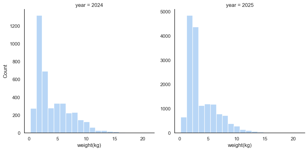
As in the previous analysis, it makes sense to stop here and appreciate just how rare those big fish are. Note that the count on the y-axis is different – there were many more catches in 2025, since the 2024 season was stopped in June, many places.

As before, we have a lot of rivers in our data set and we aren't going to be analyzing all of them:

sns.countplot(
    data=df.assign(
        size_kg=pd.cut(df["weight(kg)"], bins=[0, 7, 25], right=True)
    ),
    y="river", hue="size_kg"
).set_title("Number of salmon caught by river");

This time, I want to include Nidelva since I moved to Trondheim last year. From previous years, we know that this data set is very sparse before 2015, so we'll cut out everything prior to 2015:

df = df.loc[
    df.river.isin({"Orkla", "Gaula", "Namsenvassdraget", "Stjørdalselva", "Nidelva i Trondheim"}) & (df.year >= 2015)
].assign(
    river=lambda df: df.river.cat.remove_unused_categories(),
)

sns.relplot(
    df.groupby(
        ['river', 'year'],
        observed=False, as_index=False
    ).size().rename(columns={"size": "catches"}),
    x="year", y="catches",
    col="river", kind="line", col_wrap=3
);

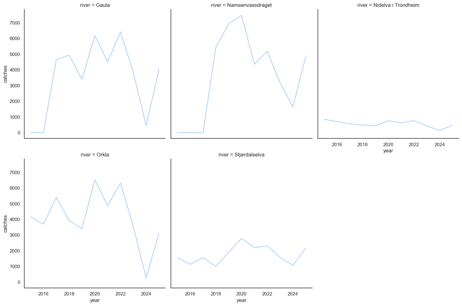
It's easy to see that 2025 at the very least resulted in more catch in all the rivers we have data for. It looks particularly dramatic in Gaula and Orkla, which were both closed in june 2024 and didn't reopen until 2025. Now let's try comparing seasons:

season_start = df.date.dt.strftime("%Y-06-01").astype('datetime64[ns]')

df = df.assign(
    day_of_season=(df.date - season_start).dt.days,
    size=lambda df: np.where(df["weight(kg)"] >= 7, "over 7kg", "under 7kg"),
    season=lambda df: np.where(df.year == 2024, "2024", np.where(df.year == 2025, "2025", "before 2024")),
)

# Historical data: group by year to get confidence interval
historical = df.loc[df.season == "before 2024"].groupby(
    ["river", "day_of_season", "size", "season", "year"], observed=False
).size().rename("catches").reset_index()

# Recent seasons: no year grouping needed, just fill missing days with 0
recent = df.loc[df.season.isin(["2024", "2025"])].groupby(
    ["river", "day_of_season", "size", "season"], observed=False
).size().rename("catches").reset_index()

catches = pd.concat([historical, recent], ignore_index=True)

sns.relplot(
    catches.loc[catches.day_of_season.between(0, 91)],
    x="day_of_season", y="catches", row="size",
    col="river", kind="line", hue="season", height=4, facet_kws={"sharey": False}
);

The shaded area is a 95% confidence interval of the seasons before 2024. The closure of the 2024 season is easily visible. While people are catching fish in 2025, it's not immediately obvious that the rivers have healthier amounts of fish then.

I feel like the best way to really understand what's going on is to use a cumulative sum plot here. This is going to help us eyeball how many fish that are being caught overall at throughout the season in a really good way, so we can see if there's a big difference between 2024 and 2025.

catches = df.groupby(
    ["river", "year", "day_of_season", "size", "season"], observed=True
).size().rename("catches").reset_index().sort_values(by="day_of_season")

catches = catches.assign(
    catches=catches.groupby(["river", "year", "size", "season"], observed=True)["catches"].cumsum()
)
catches = catches.loc[catches.day_of_season.between(0, 30)]

sns.relplot(
    catches.astype({'year': 'string'}), x="day_of_season", y="catches", row="size",
    col="river", kind="line", hue="season", height=4, facet_kws={"sharey": False}
).set_ylabels("Cumulative catches");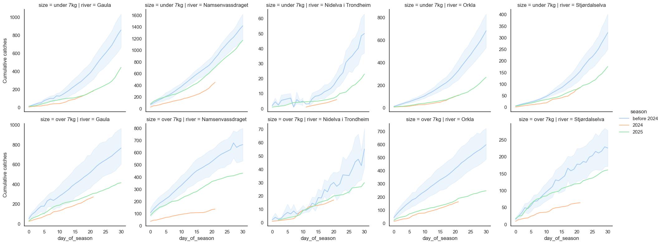

Ouch. Compared to seasons before 2024, the start of 2025 was also a terrible season in all the rivers except Namsen and perhaps Nidelva. I think these charts suggest that things aren't looking much better than in the 2024 disaster season. Let's do this plot again, without 2024 in it and including the whole season:

catches = df.groupby(
    ["river", "year", "day_of_season", "size", "season"], observed=True
).size().rename("catches").reset_index().sort_values(by="day_of_season")

catches = catches.assign(
    catches=catches.groupby(["river", "year", "size", "season"], observed=True)["catches"].cumsum()
)
catches = catches.loc[catches.day_of_season.between(0, 91) & (catches.year != 2024)]

sns.relplot(
    catches.astype({'year': 'string'}), x="day_of_season", y="catches", row="size",
    col="river", kind="line", hue="season", height=4, facet_kws={"sharey": False}
).set_ylabels("Cumulative catches");

Ah, maybe the season got off to a rocky start and improved later on. It still doesn't look good, especially not for big salmon over 7kg. We're way outside the 95% confidence interval in all the rivers for those. It doesn't look as bad for the fish under 7kg. Maybe a sign that fish aren't staying in the sea for quite as many years as before, or an effect of drought a few years back or something like that? Either way, it certainly looks like we should be paying attention for the next few years too.